Note

This page was generated from CD4_Tutorial.ipynb. Interactive online version: .

Demo: Transcriptional Patterns in CD4 T Cells#

This demo uses public data from 10x Genomics

5k Peripheral blood mononuclear cells (PBMCs) from a healthy donor with cell surface proteins (Next GEM)

as processed by Cell Ranger 3.1.0
Dataset Link

For this demo, you need the filtered h5 file, “Feature / cell matrix HDF5 (filtered)”, with the filename:

5k_pbmc_protein_v3_filtered_feature_bc_matrix.h5

Covered Here#

Data preprocessing and filtering
Computing Autocorrelation in Hotspot to identify lineage-related genes
Computing local correlations between lineage genes to identify heritable modules
Plotting modules, correlations, and module scores

[1]:

import sys

#if branch is stable, will install via pypi, else will install from source
branch = "master"
IN_COLAB = "google.colab" in sys.modules

if IN_COLAB:
    !pip install --quiet --upgrade jsonschema
    !pip install --quiet git+https://github.com/yoseflab/hotspot@$branch#egg=hotspot
    !pip install --quiet scanpy
    !pip install --quiet muon
    !pip install mplscience

     |████████████████████████████████| 72 kB 843 kB/s
ERROR: pip's dependency resolver does not currently take into account all the packages that are installed. This behaviour is the source of the following dependency conflicts.
nbclient 0.5.10 requires jupyter-client>=6.1.5, but you have jupyter-client 5.3.5 which is incompatible.
     |████████████████████████████████| 91 kB 4.3 MB/s
  Building wheel for hotspot (setup.py) ... done
     |████████████████████████████████| 2.0 MB 8.9 MB/s
     |████████████████████████████████| 86 kB 4.1 MB/s
     |████████████████████████████████| 1.1 MB 29.4 MB/s
     |████████████████████████████████| 63 kB 2.0 MB/s
  Building wheel for umap-learn (setup.py) ... done
  Building wheel for pynndescent (setup.py) ... done
  Building wheel for sinfo (setup.py) ... done
     |████████████████████████████████| 287 kB 7.6 MB/s
     |████████████████████████████████| 41 kB 115 kB/s
     |████████████████████████████████| 48 kB 4.3 MB/s
  Building wheel for loompy (setup.py) ... done
  Building wheel for numpy-groupies (setup.py) ... done
Collecting mplscience
  Downloading mplscience-0.0.5-py3-none-any.whl (4.8 kB)
Requirement already satisfied: seaborn in /usr/local/lib/python3.7/dist-packages (from mplscience) (0.11.2)
Requirement already satisfied: matplotlib in /usr/local/lib/python3.7/dist-packages (from mplscience) (3.2.2)
Collecting importlib-metadata<2.0,>=1.0
  Downloading importlib_metadata-1.7.0-py2.py3-none-any.whl (31 kB)
Requirement already satisfied: zipp>=0.5 in /usr/local/lib/python3.7/dist-packages (from importlib-metadata<2.0,>=1.0->mplscience) (3.7.0)
Requirement already satisfied: python-dateutil>=2.1 in /usr/local/lib/python3.7/dist-packages (from matplotlib->mplscience) (2.8.2)
Requirement already satisfied: pyparsing!=2.0.4,!=2.1.2,!=2.1.6,>=2.0.1 in /usr/local/lib/python3.7/dist-packages (from matplotlib->mplscience) (3.0.7)
Requirement already satisfied: kiwisolver>=1.0.1 in /usr/local/lib/python3.7/dist-packages (from matplotlib->mplscience) (1.3.2)
Requirement already satisfied: cycler>=0.10 in /usr/local/lib/python3.7/dist-packages (from matplotlib->mplscience) (0.11.0)
Requirement already satisfied: numpy>=1.11 in /usr/local/lib/python3.7/dist-packages (from matplotlib->mplscience) (1.21.5)
Requirement already satisfied: six>=1.5 in /usr/local/lib/python3.7/dist-packages (from python-dateutil>=2.1->matplotlib->mplscience) (1.15.0)
Requirement already satisfied: pandas>=0.23 in /usr/local/lib/python3.7/dist-packages (from seaborn->mplscience) (1.3.5)
Requirement already satisfied: scipy>=1.0 in /usr/local/lib/python3.7/dist-packages (from seaborn->mplscience) (1.4.1)
Requirement already satisfied: pytz>=2017.3 in /usr/local/lib/python3.7/dist-packages (from pandas>=0.23->seaborn->mplscience) (2018.9)
Installing collected packages: importlib-metadata, mplscience
  Attempting uninstall: importlib-metadata
    Found existing installation: importlib-metadata 4.11.0
    Uninstalling importlib-metadata-4.11.0:
      Successfully uninstalled importlib-metadata-4.11.0
ERROR: pip's dependency resolver does not currently take into account all the packages that are installed. This behaviour is the source of the following dependency conflicts.
markdown 3.3.6 requires importlib-metadata>=4.4; python_version < "3.10", but you have importlib-metadata 1.7.0 which is incompatible.
Successfully installed importlib-metadata-1.7.0 mplscience-0.0.5

[2]:

# download the data
if IN_COLAB:
    !wget https://cf.10xgenomics.com/samples/cell-exp/3.1.0/5k_pbmc_protein_v3_nextgem/5k_pbmc_protein_v3_nextgem_filtered_feature_bc_matrix.h5

--2022-02-18 18:00:14--  https://cf.10xgenomics.com/samples/cell-exp/3.1.0/5k_pbmc_protein_v3_nextgem/5k_pbmc_protein_v3_nextgem_filtered_feature_bc_matrix.h5
Resolving cf.10xgenomics.com (cf.10xgenomics.com)... 104.18.0.173, 104.18.1.173, 2606:4700::6812:ad, ...
Connecting to cf.10xgenomics.com (cf.10xgenomics.com)|104.18.0.173|:443... connected.
HTTP request sent, awaiting response... 200 OK
Length: 18083112 (17M) [binary/octet-stream]
Saving to: ‘5k_pbmc_protein_v3_nextgem_filtered_feature_bc_matrix.h5’

5k_pbmc_protein_v3_ 100%[===================>]  17.25M  44.4MB/s    in 0.4s

2022-02-18 18:00:14 (44.4 MB/s) - ‘5k_pbmc_protein_v3_nextgem_filtered_feature_bc_matrix.h5’ saved [18083112/18083112]

[3]:

import warnings; warnings.simplefilter('ignore')

import hotspot
import scanpy as sc
import muon as mu

import numpy as np
import mplscience

Load data from h5 file and extract CD4 T cells#

[4]:

mdata = mu.read_10x_h5("/content/5k_pbmc_protein_v3_nextgem_filtered_feature_bc_matrix.h5")

Variable names are not unique. To make them unique, call `.var_names_make_unique`.
Variable names are not unique. To make them unique, call `.var_names_make_unique`.

[5]:

mdata.var_names_make_unique()

[6]:

mdata

[6]:

MuData object with n_obs × n_vars = 5527 × 33570
  var:      'feature_types', 'gene_ids', 'genome'
  2 modalities
    rna:    5527 x 33538
      var:  'gene_ids', 'feature_types', 'genome'
    prot:   5527 x 32
      var:  'gene_ids', 'feature_types', 'genome'

[7]:

adata = mdata.mod["rna"]

[8]:

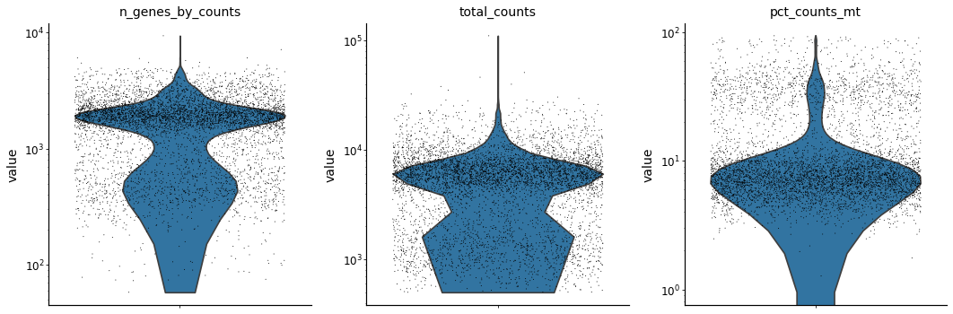
adata.var['mt'] = adata.var_names.str.startswith('MT-')  # annotate the group of mitochondrial genes as 'mt'
sc.pp.calculate_qc_metrics(adata, qc_vars=['mt'], percent_top=None, log1p=False, inplace=True)

[9]:

with mplscience.style_context():
    sc.pl.violin(adata, ['n_genes_by_counts', 'total_counts', 'pct_counts_mt'],
                jitter=0.4, multi_panel=True, log=True)

... storing 'feature_types' as categorical
... storing 'genome' as categorical

Extract the CD4 T Cells based on surface protein abundance#

[10]:

from muon import prot as pt
pt.pp.clr(mdata['prot'])

prot_data = mdata.mod["prot"]

[11]:

with mplscience.style_context():
    sc.pl.violin(prot_data, keys=["CD14_TotalSeqB", "CD4_TotalSeqB", "CD3_TotalSeqB"], multi_panel=True)

... storing 'feature_types' as categorical
... storing 'genome' as categorical

[12]:

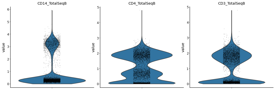
# now create a CD4 T cell mask
is_cd4 = np.asarray(
    (prot_data[:, 'CD14_TotalSeqB'].X.A < 2) &
    (prot_data[:, 'CD4_TotalSeqB'].X.A > 1) &
    (prot_data[:, 'CD3_TotalSeqB'].X.A > 1)
).ravel()

adata_cd4 = adata[is_cd4]
sc.pp.filter_cells(adata_cd4, min_genes=1000)
sc.pp.filter_genes(adata_cd4, min_cells=10)
adata_cd4 = adata_cd4[adata_cd4.obs.pct_counts_mt < 16].copy()

adata_cd4

Trying to set attribute `.obs` of view, copying.

[12]:

AnnData object with n_obs × n_vars = 1547 × 12456
    obs: 'n_genes_by_counts', 'total_counts', 'total_counts_mt', 'pct_counts_mt', 'n_genes'
    var: 'gene_ids', 'feature_types', 'genome', 'mt', 'n_cells_by_counts', 'mean_counts', 'pct_dropout_by_counts', 'total_counts', 'n_cells'

Compute a Latent Space with PCA#

In the Hotspot manuscript, we used scVI for this which has improved performance over PCA. However, to make this notebook easier to run (with less added extra dependencies), we’ll just run PCA using scanpy.

[13]:

adata_cd4.layers["counts"] = adata_cd4.X.copy()
sc.pp.normalize_total(adata_cd4)
sc.pp.log1p(adata_cd4)
adata_cd4.layers["log_normalized"] = adata_cd4.X.copy()
sc.pp.scale(adata_cd4)
sc.tl.pca(adata_cd4)

[14]:

with mplscience.style_context():
    sc.pl.pca_variance_ratio(adata_cd4)

[15]:

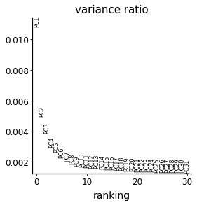
# rerun with fewer components
sc.tl.pca(adata_cd4, n_comps=10)

Creating the Hotspot object#

To start an analysis, first create the hotspot object When creating the object, you need to specify:

The gene counts matrix
Which background model to use
The latent space we are using to compute our cell metric
- Here we use the reduced, PCA results
The per-cell scaling factor
- Here we use the number of umi per barcode

In the Hotspot publication, we use the raw counts and the negative binomial (‘danb’) model. We repeat that choice here.

Once the object is created, the neighborhood is then computed with create_knn_graph

The two options that are specificied are n_neighbors which determines the size of the neighborhood, and weighted_graph.

Here we set weighted_graph=False to just use binary, 0-1 weights (only binary weights are supported when using a lineage tree) and n_neighbors=30 to create a local neighborhood size of the nearest 30 cells. Larger neighborhood sizes can result in more robust detection of correlations and autocorrelations at a cost of missing more fine-grained, smaller-scale patterns.

[16]:

# Create the Hotspot object and the neighborhood graph
# hotspot works a lot faster with a csc matrix!
adata_cd4.layers["counts_csc"] = adata_cd4.layers["counts"].tocsc()
hs = hotspot.Hotspot(
    adata_cd4,
    layer_key="counts_csc",
    model='danb',
    latent_obsm_key="X_pca",
    umi_counts_obs_key="total_counts"
)

hs.create_knn_graph(
    weighted_graph=False, n_neighbors=30,
)

Determining informative genes#

Now we compute autocorrelations for each gene, in the pca-space, to determine which genes have the most informative variation.

[17]:

hs_results = hs.compute_autocorrelations(jobs=4)

hs_results.head(15)

100%|██████████| 12456/12456 [00:09<00:00, 1313.64it/s]

[17]:

	C	Z	Pval	FDR
Gene
GZMH	0.664524	141.517601	0.0	0.0
B2M	0.637732	126.077766	0.0	0.0
RPS3A	0.679940	119.654615	0.0	0.0
CCL5	0.602698	118.413519	0.0	0.0
GZMA	0.613364	106.382416	0.0	0.0
NKG7	0.770962	106.305566	0.0	0.0
RPS13	0.583559	103.431142	0.0	0.0
RPL32	0.643652	99.413033	0.0	0.0
GZMK	0.438507	95.198094	0.0	0.0
RPS23	0.575949	94.937554	0.0	0.0
SH3BGRL3	0.511047	93.571867	0.0	0.0
CST7	0.640726	93.401829	0.0	0.0
RPS6	0.553925	90.259386	0.0	0.0
RPL30	0.599826	88.749391	0.0	0.0
MALAT1	0.518834	88.119908	0.0	0.0

Grouping genes into lineage-based modules#

To get a better idea of what expression patterns exist, it is helpful to group the genes into modules.

Hotspot does this using the concept of “local correlations” - that is, correlations that are computed between genes between cells in the same neighborhood.

Here we avoid running the calculation for all Genes x Genes pairs and instead only run this on genes that have significant autocorrelation to begin with.

The method compute_local_correlations returns a Genes x Genes matrix of Z-scores for the significance of the correlation between genes. This object is also retained in the hs object and is used in the subsequent steps.

[18]:

# Select the genes with significant lineage autocorrelation
hs_genes = hs_results.loc[hs_results.FDR < 0.05].sort_values('Z', ascending=False).head(500).index

# Compute pair-wise local correlations between these genes
lcz = hs.compute_local_correlations(hs_genes, jobs=4)

Computing pair-wise local correlation on 500 features...

100%|██████████| 500/500 [00:00<00:00, 11954.76it/s]
100%|██████████| 124750/124750 [00:26<00:00, 4788.62it/s]

Now that pair-wise local correlations are calculated, we can group genes into modules.

To do this, a convenience method is included create_modules which performs agglomerative clustering with two caveats:

If the FDR-adjusted p-value of the correlation between two branches exceeds fdr_threshold, then the branches are not merged.
If two branches are two be merged and they are both have at least min_gene_threshold genes, then the branches are not merged. Further genes that would join to the resulting merged module (and are therefore ambiguous) either remain unassigned (if core_only=True) or are assigned to the module with the smaller average correlations between genes, i.e. the least-dense module (if core_only=False)

The output is a Series that maps gene to module number. Unassigned genes are indicated with a module number of -1

This method was used to preserved substructure (nested modules) while still giving the analyst some control. However, since there are a lot of ways to do hierarchical clustering, you can also manually cluster using the gene-distances in hs.local_correlation_z

[19]:

modules = hs.create_modules(
    min_gene_threshold=15, core_only=True, fdr_threshold=0.05
)

modules.value_counts()

[19]:

 1     89
-1     74
 5     42
 10    35
 8     34
 3     32
 6     32
 2     30
 12    30
 11    28
 9     23
 4     18
 7     18
 13    15
Name: Module, dtype: int64

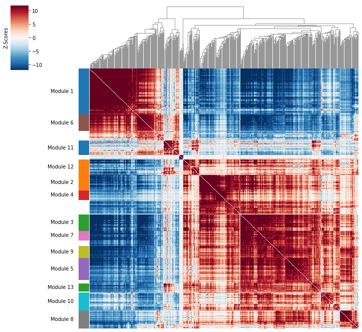
Plotting module correlations#

A convenience method is supplied to plot the results of hs.create_modules

[20]:

hs.plot_local_correlations(vmin=-12, vmax=12)

To explore individual genes, we can look at the genes with the top autocorrelation in a given module as these are likely the most informative.

[21]:

# Show the top genes for a module

module = 9

results = hs.results.join(hs.modules)
results = results.loc[results.Module == module]

results.sort_values('Z', ascending=False).head(10)

[21]:

	C	Z	Pval	FDR	Module
Gene
MIAT	0.177204	33.820983	4.847800e-251	3.531240e-249	9.0
GBP5	0.208299	32.325981	1.509384e-229	1.005395e-227	9.0
AC004687.1	0.188952	31.505214	3.684686e-218	2.378054e-216	9.0
MAF	0.187160	28.825567	5.129598e-183	2.985714e-181	9.0
NEAT1	0.232268	27.821226	1.200974e-170	6.738436e-169	9.0
PPP2R5C	0.143905	26.519352	2.899214e-155	1.517336e-153	9.0
PYHIN1	0.165599	26.442412	2.230444e-154	1.162444e-152	9.0
OPTN	0.157458	24.916422	2.469573e-137	1.206314e-135	9.0
TNFRSF1B	0.235988	24.834521	1.900423e-136	9.210766e-135	9.0
CYTOR	0.237405	23.794265	1.914537e-125	8.832399e-124	9.0

Summary Module Scores#

To aid in the recognition of the general behavior of a module, Hotspot can compute aggregate module scores.

[22]:

module_scores = hs.calculate_module_scores()

module_scores.head()

Computing scores for 13 modules...

100%|██████████| 13/13 [00:00<00:00, 15.00it/s]

[22]:

	1	2	3	4	5	6	7	8	9	10	11	12	13
AAACGAATCATGAGAA-1	3.608087	-1.332635	-2.765422	-0.375033	-1.989659	2.508126	-1.359988	-0.366706	-1.243118	-1.344597	-1.256328	-1.276302	-1.621497
AAACGCTAGGATAATC-1	5.611630	-1.164912	-2.213463	-0.401776	-1.021839	1.402271	-1.262448	-0.809071	-1.175233	-1.255394	-1.539582	-1.744215	-1.434432
AAAGAACTCTTGGTCC-1	-11.978400	-0.568684	4.818443	-0.418272	10.817546	-2.620614	4.777415	9.616011	5.739911	1.219397	-3.064364	-0.916039	0.462314
AAAGGATAGCCGGATA-1	6.380645	-1.209119	-2.518803	-0.393690	-1.559012	2.280116	-1.609583	-0.948184	-1.546197	-1.430628	0.211499	-1.771080	-0.803406
AAAGGATTCCGAGTGC-1	4.914818	-0.754171	0.405689	-0.369875	-0.676271	-1.565022	0.578168	-0.535698	-0.047888	2.093285	-3.645493	-0.315027	-1.429217

Here we can visualize these module scores by plotting them over a UMAP of the cells

First we’ll compute the UMAP

[23]:

sc.pp.neighbors(adata_cd4)
sc.tl.umap(adata_cd4)
sc.pl.umap(adata_cd4, frameon=False)

[24]:

module_cols = []
for c in module_scores.columns:
    key = f"Module {c}"
    adata_cd4.obs[key] = module_scores[c]
    module_cols.append(key)

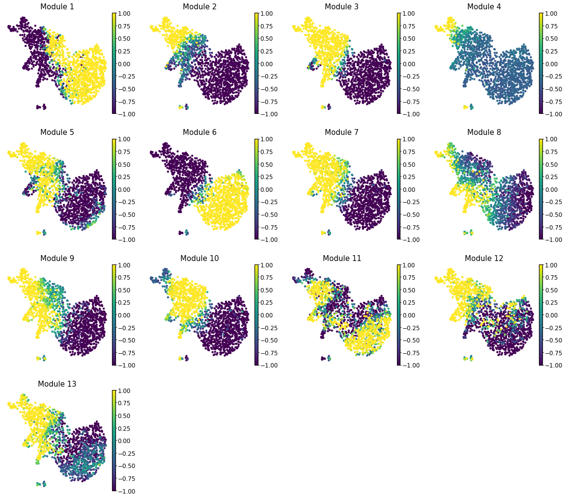
Finally, we plot the module scores on top of the UMAP for comparison

[25]:

with mplscience.style_context():
    sc.pl.umap(adata_cd4, color=module_cols, frameon=False, vmin=-1, vmax=1)

Demo: Transcriptional Patterns in CD4 T Cells

Contents

Demo: Transcriptional Patterns in CD4 T Cells#

Covered Here#

Load data from h5 file and extract CD4 T cells#

Extract the CD4 T Cells based on surface protein abundance#

Compute a Latent Space with PCA#

Creating the Hotspot object#

Determining informative genes#

Grouping genes into lineage-based modules#

Plotting module correlations#

Summary Module Scores#