Note

This page was generated from Spatial_Tutorial.ipynb. Interactive online version: .

Demo: Spatial data from Slide-seq#

This demo uses data from:

Slide-seq: A scalable technology for measuring genome-wide expression at high spatial resolution

Rodriques et al (Science 2019)
https://doi.org/10.1126/science.aaw1219

For this demo, you need the data files for Puck_180819_12

Taken from: https://portals.broadinstitute.org/single_cell/study/SCP354/slide-seq-study#study-summary

Specifically these two files:

MappedDGEForR.csv
BeadMapping_10-17_1014/BeadLocationsForR.csv

For convenience, we have wrapped this in an AnnData object that you will download below.

Covered Here#

Computing Autocorrelation in Hotspot to identify spatial genes
Computing local correlations between spatial genes to identify modules
Plotting modules, correlations, and module scores

Not Covered Here#

Data preprocessing (see Squidpy/Scanpy)

[1]:

import sys

#if branch is stable, will install via pypi, else will install from source
branch = "anndata"
IN_COLAB = "google.colab" in sys.modules

if IN_COLAB:
    !pip install --quiet --upgrade numba
    !pip install git+https://github.com/yoseflab/hotspot@$branch#egg=hotspot
    !pip install --quiet scanpy
    !pip install --quiet mplscience

     |████████████████████████████████| 3.3 MB 8.3 MB/s
     |████████████████████████████████| 34.5 MB 1.4 MB/s
Collecting hotspot
  Cloning https://github.com/yoseflab/hotspot (to revision anndata) to /tmp/pip-install-6tu2qe3n/hotspot_3d0fc0f8c2b94342ad19e622464099fe
  Running command git clone -q https://github.com/yoseflab/hotspot /tmp/pip-install-6tu2qe3n/hotspot_3d0fc0f8c2b94342ad19e622464099fe
  Running command git checkout -b anndata --track origin/anndata
  Switched to a new branch 'anndata'
  Branch 'anndata' set up to track remote branch 'anndata' from 'origin'.
Requirement already satisfied: matplotlib>=3.0.0 in /usr/local/lib/python3.7/dist-packages (from hotspot) (3.2.2)
Requirement already satisfied: numba>=0.43.1 in /usr/local/lib/python3.7/dist-packages (from hotspot) (0.55.1)
Requirement already satisfied: numpy>=1.16.4 in /usr/local/lib/python3.7/dist-packages (from hotspot) (1.21.5)
Requirement already satisfied: seaborn>=0.9.0 in /usr/local/lib/python3.7/dist-packages (from hotspot) (0.11.2)
Requirement already satisfied: scipy>=1.2.1 in /usr/local/lib/python3.7/dist-packages (from hotspot) (1.4.1)
Requirement already satisfied: pandas>=0.24.0 in /usr/local/lib/python3.7/dist-packages (from hotspot) (1.3.5)
Requirement already satisfied: tqdm>=4.32.2 in /usr/local/lib/python3.7/dist-packages (from hotspot) (4.62.3)
Requirement already satisfied: statsmodels>=0.9.0 in /usr/local/lib/python3.7/dist-packages (from hotspot) (0.10.2)
Requirement already satisfied: scikit-learn>=0.21.2 in /usr/local/lib/python3.7/dist-packages (from hotspot) (1.0.2)
Collecting anndata>=0.7
  Downloading anndata-0.7.8-py3-none-any.whl (91 kB)
     |████████████████████████████████| 91 kB 4.3 MB/s
Requirement already satisfied: importlib_metadata>=0.7 in /usr/local/lib/python3.7/dist-packages (from anndata>=0.7->hotspot) (4.11.0)
Requirement already satisfied: xlrd<2.0 in /usr/local/lib/python3.7/dist-packages (from anndata>=0.7->hotspot) (1.1.0)
Requirement already satisfied: h5py in /usr/local/lib/python3.7/dist-packages (from anndata>=0.7->hotspot) (3.1.0)
Requirement already satisfied: packaging>=20 in /usr/local/lib/python3.7/dist-packages (from anndata>=0.7->hotspot) (21.3)
Requirement already satisfied: natsort in /usr/local/lib/python3.7/dist-packages (from anndata>=0.7->hotspot) (5.5.0)
Requirement already satisfied: zipp>=0.5 in /usr/local/lib/python3.7/dist-packages (from importlib_metadata>=0.7->anndata>=0.7->hotspot) (3.7.0)
Requirement already satisfied: typing-extensions>=3.6.4 in /usr/local/lib/python3.7/dist-packages (from importlib_metadata>=0.7->anndata>=0.7->hotspot) (3.10.0.2)
Requirement already satisfied: pyparsing!=2.0.4,!=2.1.2,!=2.1.6,>=2.0.1 in /usr/local/lib/python3.7/dist-packages (from matplotlib>=3.0.0->hotspot) (3.0.7)
Requirement already satisfied: cycler>=0.10 in /usr/local/lib/python3.7/dist-packages (from matplotlib>=3.0.0->hotspot) (0.11.0)
Requirement already satisfied: kiwisolver>=1.0.1 in /usr/local/lib/python3.7/dist-packages (from matplotlib>=3.0.0->hotspot) (1.3.2)
Requirement already satisfied: python-dateutil>=2.1 in /usr/local/lib/python3.7/dist-packages (from matplotlib>=3.0.0->hotspot) (2.8.2)
Requirement already satisfied: setuptools in /usr/local/lib/python3.7/dist-packages (from numba>=0.43.1->hotspot) (57.4.0)
Requirement already satisfied: llvmlite<0.39,>=0.38.0rc1 in /usr/local/lib/python3.7/dist-packages (from numba>=0.43.1->hotspot) (0.38.0)
Requirement already satisfied: pytz>=2017.3 in /usr/local/lib/python3.7/dist-packages (from pandas>=0.24.0->hotspot) (2018.9)
Requirement already satisfied: six>=1.5 in /usr/local/lib/python3.7/dist-packages (from python-dateutil>=2.1->matplotlib>=3.0.0->hotspot) (1.15.0)
Requirement already satisfied: threadpoolctl>=2.0.0 in /usr/local/lib/python3.7/dist-packages (from scikit-learn>=0.21.2->hotspot) (3.1.0)
Requirement already satisfied: joblib>=0.11 in /usr/local/lib/python3.7/dist-packages (from scikit-learn>=0.21.2->hotspot) (1.1.0)
Requirement already satisfied: patsy>=0.4.0 in /usr/local/lib/python3.7/dist-packages (from statsmodels>=0.9.0->hotspot) (0.5.2)
Requirement already satisfied: cached-property in /usr/local/lib/python3.7/dist-packages (from h5py->anndata>=0.7->hotspot) (1.5.2)
Building wheels for collected packages: hotspot
  Building wheel for hotspot (setup.py) ... done
  Created wheel for hotspot: filename=hotspot-0.9.1-py3-none-any.whl size=25699 sha256=32673675d4f8d6d438cf928d204c37d679c313816ab5132f7cd71ee8958ad92f
  Stored in directory: /tmp/pip-ephem-wheel-cache-5a1kxpla/wheels/5f/06/1e/4c02025a303d8ff93d24e7c0d16a570a6b7da858ddf9680c63
Successfully built hotspot
Installing collected packages: anndata, hotspot
Successfully installed anndata-0.7.8 hotspot-0.9.1
     |████████████████████████████████| 2.0 MB 8.5 MB/s
     |████████████████████████████████| 86 kB 5.3 MB/s
     |████████████████████████████████| 1.1 MB 64.6 MB/s
     |████████████████████████████████| 63 kB 1.8 MB/s
  Building wheel for umap-learn (setup.py) ... done
  Building wheel for pynndescent (setup.py) ... done
  Building wheel for sinfo (setup.py) ... done
ERROR: pip's dependency resolver does not currently take into account all the packages that are installed. This behaviour is the source of the following dependency conflicts.
markdown 3.3.6 requires importlib-metadata>=4.4; python_version < "3.10", but you have importlib-metadata 1.7.0 which is incompatible.

[2]:

import scanpy as sc
import hotspot

import numpy as np
import mplscience
import matplotlib

/usr/local/lib/python3.7/dist-packages/statsmodels/tools/_testing.py:19: FutureWarning: pandas.util.testing is deprecated. Use the functions in the public API at pandas.testing instead.
  import pandas.util.testing as tm

[ ]:

url = "https://github.com/YosefLab/scVI-data/blob/master/rodriques_slideseq.h5ad?raw=true"
adata = sc.read("rodriques_slideseq.h5ad", backup_url=url)
adata.obs["total_counts"] = np.asarray(adata.X.sum(1)).ravel()

adata.layers["csc_counts"] = adata.X.tocsc()

# renormalize the data for expression viz on plots
sc.pp.normalize_total(adata)
sc.pp.log1p(adata)

Creating the Hotspot object#

To start an analysis, first creat the hotspot object When creating the object, you need to specify:

The gene counts matrix
Which background model to use
The latent space we are using to compute our cell metric
- Here we use the physical barcode positions
The per-cell scaling factor
- Here we use the number of umi per barcode

Once the object is created, the neighborhood graph must be computed with create_knn_graph

The two options that are specificied are n_neighbors which determines the size of the neighborhood, and weighted_graph.

Here we set weighted_graph=False to just use binary, 0-1 weights and n_neighbors=300 to create a local neighborhood size of the nearest 300 barcodes. Larger neighborhood sizes can result in more robust detection of correlations and autocorrelations at a cost of missing more fine-grained, smaller-scale, spatial patterns

[5]:

# Create the Hotspot object and the neighborhood graph
hs = hotspot.Hotspot(
    adata,
    layer_key="csc_counts",
    model='bernoulli',
    latent_obsm_key="spatial",
    umi_counts_obs_key="total_counts",
)

hs.create_knn_graph(
    weighted_graph=False, n_neighbors=300,
)

Determining genes with spatial variation#

Now we compute autocorrelations for each gene, using the spatial metric, to determine which genes have the most spatial variation.

[6]:

hs_results = hs.compute_autocorrelations(jobs=4)

hs_results.head()

100%|██████████| 6942/6942 [06:36<00:00, 17.53it/s]

[6]:

	C	Z	Pval	FDR
Gene
Ttr	0.198161	438.058454	0.0	0.0
Plp1	0.110854	246.179606	0.0	0.0
Enpp2	0.103074	211.241807	0.0	0.0
Fth1	0.092905	207.076233	0.0	0.0
Cartpt	0.087053	180.180043	0.0	0.0

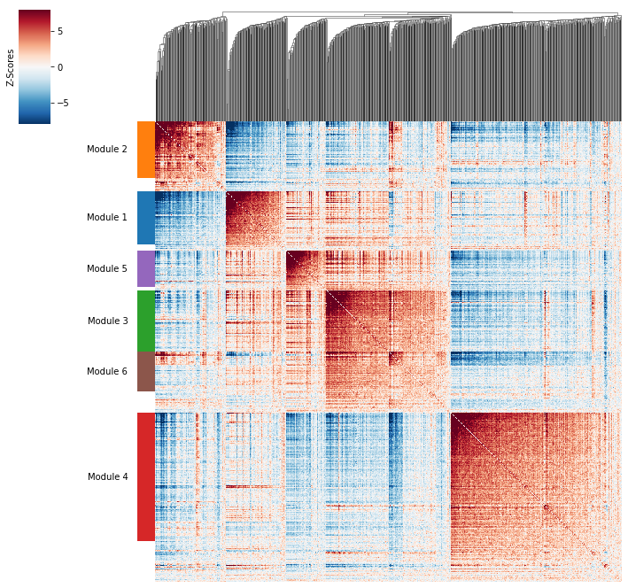
Grouping genes into spatial modules#

To get a better idea of what spatial patterns exist, it is helpful to group the genes into modules.

Hotspot does this using the concept of “local correlations” - that is, correlations that are computed between genes between cells in the same neighborhood.

Here we avoid running the calculation for all Genes x Genes pairs and instead only run this on genes that have significant spatial autocorrelation to begin with.

The method compute_local_correlations returns a Genes x Genes matrix of Z-scores for the significance of the correlation between genes. This object is also retained in the hs object and is used in the subsequent steps.

[7]:

# Select the genes with significant spatial autocorrelation
hs_genes = hs_results.index[hs_results.FDR < 0.05]

# Compute pair-wise local correlations between these genes
lcz = hs.compute_local_correlations(hs_genes, jobs=4)

Computing pair-wise local correlation on 876 features...

100%|██████████| 876/876 [00:07<00:00, 110.16it/s]
100%|██████████| 383250/383250 [4:00:06<00:00, 26.60it/s]

Now that pair-wise local correlations are calculated, we can group genes into modules.

To do this, a convenience method is included create_modules which performs agglomerative clustering with two caveats:

If the FDR-adjusted p-value of the correlation between two branches exceeds fdr_threshold, then the branches are not merged.
If two branches are two be merged and they are both have at least min_gene_threshold genes, then the branches are not merged. Further genes that would join to the resulting merged module (and are therefore ambiguous) either remain unassigned (if core_only=True) or are assigned to the module with the smaller average correlations between genes, i.e. the least-dense module (if core_only=False)

The output is a Series that maps gene to module number. Unassigned genes are indicated with a module number of -1

This method was used to preserved substructure (nested modules) while still giving the analyst some control. However, since there are a lot of ways to do hierarchical clustering, you can also manually cluster using the gene-distances in hs.local_correlation_z

[8]:

modules = hs.create_modules(
    min_gene_threshold=20, core_only=False, fdr_threshold=0.05
)

modules.value_counts()

[8]:

 4    243
-1    163
 3    117
 2    108
 1    101
 6     75
 5     69
Name: Module, dtype: int64

Plotting module correlations#

A convenience method is supplied to plot the results of hs.create_modules

[9]:

hs.plot_local_correlations()

To explore individual genes, we can look at the genes with the top autocorrelation in a given module as these are likely the most informative.

[10]:

# Show the top genes for a module

module = 1

results = hs.results.join(hs.modules)
results = results.loc[results.Module == module]
results.sort_values('Z', ascending=False).head(10)

[10]:

	C	Z	Pval	FDR	Module
Gene
Plp1	0.110854	246.179606	0.000000e+00	0.000000e+00	1.0
Fth1	0.092905	207.076233	0.000000e+00	0.000000e+00	1.0
Mbp	0.059088	130.720208	0.000000e+00	0.000000e+00	1.0
Apod	0.026268	57.079755	0.000000e+00	0.000000e+00	1.0
Mobp	0.022971	50.674919	0.000000e+00	0.000000e+00	1.0
Mal	0.019166	41.898995	0.000000e+00	0.000000e+00	1.0
Trf	0.014862	32.176305	1.893429e-227	3.552483e-225	1.0
Car2	0.012635	27.513785	6.004986e-167	9.925385e-165	1.0
Cryab	0.011001	23.612011	1.450564e-123	1.974473e-121	1.0
Ermn	0.010955	22.928582	1.205287e-116	1.494125e-114	1.0

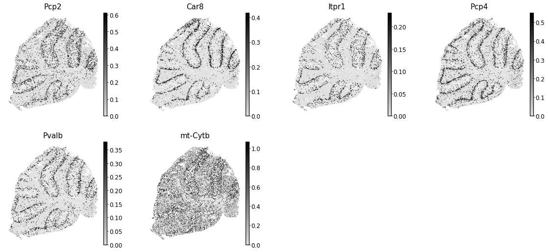
To get an idea of what spatial pattern the module is referencing, we can plot the top module genes’ expression onto the spatial positions

[38]:

cmap = matplotlib.colors.LinearSegmentedColormap.from_list(
    'grays', ['#DDDDDD', '#000000'])

module = 2
results = hs.results.join(hs.modules)
results = results.loc[results.Module == module]
genes = results.sort_values('Z', ascending=False).head(6).index

with mplscience.style_context():
    sc.pl.spatial(
        adata,
        color=genes,
        cmap=cmap,
        frameon=False,
        vmin='p0',
        vmax='p95',
        spot_size=30,
    )

Summary Module Scores#

To aid in the recognition of the general behavior of a module, Hotspot can compute aggregate module scores.

[20]:

module_scores = hs.calculate_module_scores()

module_scores.head()

Computing scores for 6 modules...

100%|██████████| 6/6 [01:24<00:00, 14.08s/it]

[20]:

	1	2	3	4	5	6
barcodes
CGTACAATTTTTTT	-0.421503	0.829196	-0.025306	-0.403850	-0.209946	0.058708
TTCGTTATTTTTTT	-0.433274	1.194746	-0.251114	-0.451753	-0.206384	0.263886
CAAACCAACCCCCC	-0.302593	0.609414	-0.171035	0.265985	-0.315975	0.350375
TCTTTTCACCCCCC	-0.510236	1.309481	-0.082019	-0.743183	-0.100390	0.198135
GGATTGAACCCCCC	-0.554569	0.108010	-0.132590	-0.338540	-0.142225	0.255825

[21]:

module_cols = []
for c in module_scores.columns:
    key = f"Module {c}"
    adata.obs[key] = module_scores[c]
    module_cols.append(key)

Here we can visualize these module scores by plotting them over the barcode positions:

[39]:

with mplscience.style_context():
    sc.pl.spatial(adata, color=module_cols, frameon=False, vmin="p0", vmax="p99", spot_size=30)

Demo: Spatial data from Slide-seq

Contents

Demo: Spatial data from Slide-seq#

Covered Here#

Not Covered Here#

Creating the Hotspot object#

Determining genes with spatial variation#

Grouping genes into spatial modules#

Plotting module correlations#

Summary Module Scores#